1 INRA, Laboratoire de génétique et
amélioration des arbres forestiers,
2 INRA, Laboratoire de Malherbologie,
*Corresponding author: Email: antoine.kremer@zouk.pierroton.inra.fr
Introduction
Measuring gene diversity within natural populations with the help of molecular markers follows a two-step sampling procedure: sampling populations and individuals, and sampling of gene loci within the genome. Most of the attention has so far been addressed to the sampling of populations and individuals. Sampling variance and confidence intervals were developed through analytical calculations and were applied for defining optimal sampling strategies (Brown and Weir, 1983).
However, sampling within the genome has received much less attention, mostly because the distribution of genetic polymorphism within the genome is largely unknown. We have addressed this problem by using simulation methods and by comparing advantages and drawbacks of different markers that have different distributions within the genome. Considering the current state of the art in genetic markers, two extreme sampling strategies can be adopted in reference to molecular markers: (1) selection of a few highly informative markers (microsatellites), (2) sampling of numerous poorly informative markers randomly distributed within the genome (AFLPs). We compared these two extreme strategies for measuring within-population diversity.
Methods
The simulation model that was developed to evaluate sampling strategies comprises three different steps. The model is inspired from METAPOP (Lecorre et al., 1996).
Step 1: Simulation of a genome
A given genome comprising 1000 loci is created once the user has introduced a number of linkage groups. The total number of loci are then equally distributed among the linkage groups. Recombination rates among loci are then calculated.
A set of loci (loci under investigation) among the 1000 can then be selected by the user corresponding to his interest. This is where the user chooses either AFLPs or microsatellites. The level of diversity will be compared between the whole genome (1000 loci) and the subset of markers he is interested in.
Step 2: Simulation of a metapopulation
A set of populations is created, which are interconnected by pollen and gene flow. The user defines the number of populations, population size and migration rates (for pollen and seed) among populations. Genomes are then generated for all of the individuals in all populations according to Step 1.
Step 3: Simulation of an evolutionary scenario
Various genetic processes can be introduced in the simulation model:
The simulation proceeds as follows:
At each generation, Nei's genetic diversity is calculated for the three different set of markers in each population:
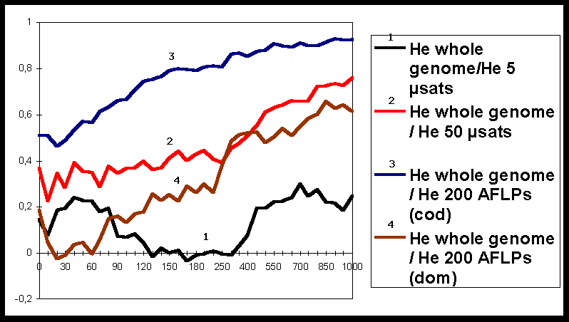
Simulations were conducted in a case study corresponding to a simplified situation in forest trees. The input parameters for METAPOP are indicated in Table 1. For a given scenario, simulations were repeated 10 times to account for stochastic variation. The values of diversity were recorded for each marker (and the whole genome) and after each generation. Correlation coefficients were computed for diversity He calculated over the whole genome and diversity assessed with the different markers.
The results (Figure 1) clearly show that during a few hundreds of generations these correlations remain low, whatever the markers are. These results indicate that, when populations are not under equilibrium between migration-drift and mutation, there can be a substantial discrepancy between diversity assessed with markers and diversity over the whole genome.
When populations tended towards equilibrium, correlation steadily increased. Furthermore, diversity estimated with 200 AFLP dominant markers is as efficient as diversity measured with 50 codominant microsatellite loci. These results clearly show that there is a trade-off between number of loci and precision of information at each locus.
Finally, Figure 1 also shows how the assessment at a reduced number of loci can be misleading: there is an important discrepancy between diversity estimates made on 5 microsatellite loci and on the whole genome.
References
Brown AHD, Weir BS (1983) Measuring genetic variability in plant populations. In: Tanksley SD, Orton TJ (eds.). Isozymes in Plant Genetics and Breeding, Part A. Elsevier, pp. 219-239.
Lecorre V, Machon N, Petit RJ, Kremer A (1997) Colonization with long-distance seed dispersal and genetic structure of maternally inherited genes in forest trees: a simulation study. Genet. Res, Camb. 69: 117-125.
|
|
|
|
|
|
Total genome | 1000 loci and 10 linkage groups
Mutation rate for each locus : 10-6 |
| AFLPs | 200 loci (mutation rate 10-6), 20
on each linkage group.
Mutation rate for each locus : 10-6 |
|
| Microsatellites | 5 loci (1 on 5 linkage groups)
50 loci (5 on each linkage group) Mutation rate 10-3 |
|
| Simulation of a metapopulation | Number of populations | 25 |
| Population size | 1000 | |
| Pollen migration rate | 0.01 | |
| Seed dispersion rate | 0.0001 | |
| Gene flow model | Two dimensional stepping stone | |
| Simulation of an evolutionary scenario | Selection | No selection |
| Demography | Populations reached population size in one generation | |
| Extinction | No extinction | |

Figure 1: Evolution of correlation coefficients between genetic diversity at the whole genome and genetic diversity for different types of markers. The X-axis represents the number of generations.
© Institut für Forstgenetik und Forstpflanzenzüchtung, Universität Göttingen, 1999